Grid sequencing¶

The previous sections were not very ambitious. We were just getting started! Now we demonstrate a serious PISM capability, the ability to change, specifically to refine, the grid resolution at runtime.

One can of course do the longest model runs using a coarse grid, like the 20 km grid used first. It is, however, only possible to pick up detail from high quality data, for instance bed elevation and high-resolution climate data, using high grid resolution.

A 20 or 10 km grid is inadequate for resolving the flow of the ice sheet through the kind of fjord-like, few-kilometer-wide topographical confinement which occurs, for example, at Jakobshavn Isbrae in the west Greenland ice sheet [33], an important outlet glacier which both flows fast and drains a large fraction of the ice sheet. One possibility is to set up an even higher-resolution PISM regional model covering only one outlet glacier, but this requires decisions about coupling to the whole ice sheet flow. (See section Example: A regional model of the Jakobshavn outlet glacier in Greenland.) Here we will work on high resolution for the whole ice sheet, and thus all outlet glaciers.

Consider the following command and compare it to the first one:

mpiexec -n 4 pismr \
        -bootstrap -i pism_Greenland_5km_v1.1.nc \
        -Mx 301 -My 561 \
        -Mz 201 -Lz 4000 -z_spacing equal \
        -Mbz 21 -Lbz 2000 \
        -ys -200 -ye 0 \
        -regrid_file g20km_10ka_hy.nc \
        -regrid_vars litho_temp,thk,enthalpy,tillwat,bmelt ...

Instead of a 20 km grid in the horizontal (-Mx 76 -My 141) we ask for a 5 km grid (-Mx 301 -My 561). Instead of vertical grid resolution of 40 m (-Mz 101 -z_spacing equal -Lz 4000) we ask for a vertical resolution of 20 m (-Mz 201 -z_spacing equal -Lz 4000).1 Most significantly, however, we say -regrid_file g20km_10ka_hy.nc to regrid — specifically, to bilinearly-interpolate — fields from a model result computed on the coarser 20 km grid. The regridded fields (-regrid_vars litho_temp,...) are the evolving mass and energy state variables which are already approximately at equilibrium on the coarse grid. Because we are bootstrapping (i.e. using the -bootstrap option), the other variables, especially the bedrock topography topg and the climate data, are brought in to PISM at “full” resolution, that is, on the original 5 km grid in the data file pism_Greenland_5km_v1.1.nc.

This technique could be called “grid sequencing”.2

By approximating the equilibrium state on a coarser grid and then interpolating onto a finer grid the command above allows us to obtain the near-equilibrium result on the finer 5km grid using a relatively short (200 model years) run. How close to equilibrium we get depends on both durations, i.e. on both the coarse and fine grid run durations, but certainly the computational effort is reduced by doing a short run on the fine grid. Note that in the previous subsection we also used regridding. In that application, however, -regrid_file only “brings in” fields from a run on the same resolution.

Generally the fine grid run duration in grid sequencing should be at least \(t = \dx / v_{\text{min}}\) where \(\dx\) is the fine grid resolution and \(v_{\text{min}}\) is the lowest ice flow speed that we expect to be relevant to our modeling purposes. That is, the duration should be such that slow ice at least has a chance to cross one grid cell. In this case, if \(\dx = 5\) km and \(v_{\text{min}} = 25\) m/year then we get \(t=200\) a. Though we use this as the duration, it is a bit short, and the reader might compare \(t=500\) results (i.e. using \(v_{\text{min}} = 10\) m/year).

Actually we will demonstrate how to go from \(20\km\) to \(5\km\) in two steps, \(20\km\,\to\,10\km\,\to\,5\km\), with durations of \(10000\), \(2000\), and \(200\) years, respectively. The 20 km coarse grid run is already done; the result is in g20km_10ka_hy.nc. So we run the following script which is gridseq.sh in examples/std-greenland/. It calls spinup.sh to collect all the right PISM options:

#!/bin/bash
NN=4
export PARAM_PPQ=0.5
export REGRIDFILE=g20km_10ka_hy.nc
export EXSTEP=100
./spinup.sh $NN const 2000  10 hybrid g10km_gridseq.nc
export REGRIDFILE=g10km_gridseq.nc
export EXSTEP=10
./spinup.sh $NN const 200    5 hybrid  g5km_gridseq.nc

Environment variable EXSTEP specifies the time in years between writing the spatially-dependent, and large-file-size-generating, frames for the -extra_file ... diagnostic output.

Warning

The 5 km run requires 8 Gb of memory at minimum!

If you try it without at least 8 Gb of memory then your machine will “bog down” and start using the hard disk for swap space! The run will not complete and your hard disk will get a lot of wear! (If you have less than 8 Gb memory, comment out the last three lines of the above script by putting the “#” character at the beginning of the line so that you only do the 20 km \(\to\) 10 km refinement.)

Run the script like this:

./gridseq.sh &> out.gridseq &

The 10 km run takes under two wall-clock hours (8 processor-hours) and the 5 km run takes about 6 wall-clock hours (24 processor-hours).

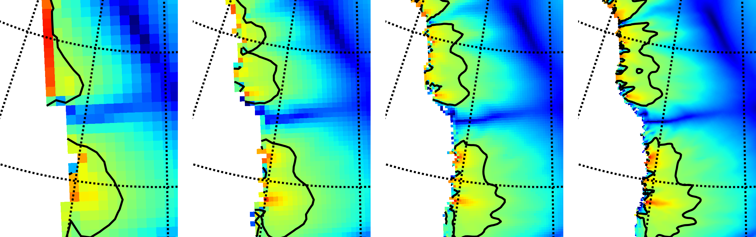
../../_images/g40-20-10-5km-detail.png — Fig. 10 Detail of field `velsurf_mag` showing the central western coast of Greenland, including Jakobshavn Isbrae (lowest major flow), from runs of resolution 40, 20, 10, 5 km (left-to-right). Color scheme and scale, including 100 m/year contour (solid black), are all identical to `velsurf_mag` Figures Fig. 4, Fig. 5, and Fig. 6.¶

Fig. 10, showing only a detail of the western coast of Greenland, with several outlet glaciers visible, suggests what is accomplished: the high resolution runs have separated outlet glacier flows, as they are in reality. Note that all of these results were generated in a few wall clock hours on a laptop! The surface speed velsurf_mag from files g10km_gridseq.nc and g5km_gridseq.nc is shown (two right-most subfigures). In the two left-hand subfigures we show the same field from NetCDF files g40km_10ka_hy.nc and g20km_10ka_hy.nc; the former is an added 40 km result using an obvious modification of the run in section Second run: a better ice-dynamics model.

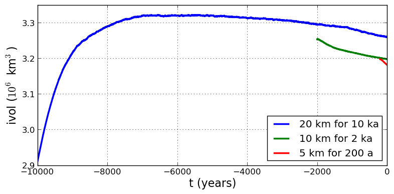
../../_images/ivol-gridseq.png — Fig. 11 Time series of ice volume `ice_volume_glacierized` from the three runs in our grid sequencing example: 20 km for 10 ka = `ts_g20km_10ka_hy.nc`, 10 km for 2 ka = `ts_g10km_gridseq.nc`, and 5 km for 200 a = `ts_g5km_gridseq.nc`.¶

Fig. 11, which shows time series of ice volume, also shows the cost of high resolution, however. The short 200 a run on the 5 km grid took about 3 wall-clock hours compared to the 10 minutes taken by the 10 ka run on a 20 km grid. The fact that the time series for ice volume on 10 km and 5 km grids are not very “steady” also suggests that these runs should actually be longer.

In this vein, if you have an available supercomputer then a good exercise is to extend our grid sequencing example to 3 km or 2 km resolutions [2]; these grids are already supported in the script spinup.sh. Note that the vertical grid also generally gets refined as the horizontal grid is refined.

Going to a 1km grid is possible, but you will start to see the limitations of distributed file systems in writing the enormous NetCDF files in question [11]. Notice that a factor-of-five refinement in all three dimensions, e.g. from 5 km to 1 km in the horizontal, and from 20 m to 4 m in the vertical, generates an output NetCDF file which is 125 times larger. Since the already-generated 5 km result g5km_gridseq.nc is over 0.5 Gb, the result is a very large file at 1 km.

On the other hand, on fine grids we observe that memory parallelism, i.e. spreading the stored model state over the separated memory of many nodes of supercomputers, is as important as the usual computation (CPU) parallelism.

This subsection has emphasized the “P” in PISM, the nontrivial parallelism in which the solution of the conservation equations, especially the stress balance equations, is distributed across processors. An easier and more common mode of parallelism is to distribute distinct model runs, each with different parameter values, among the processors. For scientific purposes, such parameter studies, whether parallel or not, are at least as valuable as individual high-resolution runs.

Footnotes

1: See subsections Bootstrapping, Computational box, and Spatial grid for more about determining the computation domain and grid at bootstrapping.
2: It is not quite “multigrid.” That would both involve refinement and coarsening stages in computing the fine grid solution.