Fourth run: paleo-climate model spin-up

A this point we have barely mentioned one of the most important players in an ice sheet model: the surface mass balance (SMB) model. Specifically, an SMB model combines precipitation (e.g. [29] for present-day Greenland) and a model for melt. Melt models are always based on some approximation of the energy available at the ice surface [30]. Previous runs in this section used a “constant-climate” assumption, which specifically meant using the modeled present-day SMB rates from the regional climate model RACMO [7], as contained in the SeaRISE-Greenland data set Greenland_5km_v1.1.nc.

While a physical model of ice dynamics only describes the movement of the ice, the SMB (and the sub-shelf melt rate) are key inputs which directly determine changes in the boundary geometry. Boundary geometry changes then influence the stresses seen by the stress balance model and thus the motion.

There are other methods for producing SMB than using present-day modeled values. We now try such a method, a “paleo-climate spin-up” for our Greenland ice sheet model. Of course, direct measurements of prior climates in Greenland are not available as data! There are, however, estimates of past surface temperatures at the locations of ice cores (see [8] for GRIP), along with estimates of past global sea level [9] which can be used to determine where the flotation criterion is applied—this is how PISM’s mask variable is determined. Also, models have been constructed for how precipitation differs from the present-day values [31]. For demonstration purposes, these are all used in the next run. The relevant options are further documented in the Climate Forcing Manual.

As noted, one must compute melt in order to compute SMB. Here this is done using a temperature-index, “positive degree-day” (PDD) model [30]. Such a PDD model has parameters for how much snow and/or ice is melted when surface temperatures spend time near or above zero degrees. Again, see the Climate Forcing Manual for relevant options.

To summarize the paleo-climate model applied here, temperature offsets from the GRIP core record affect the snow energy balance, and thus the rates of melting and runoff calculated by the PDD model. In warm periods there is more marginal ablation, but precipitation may also increase (according to a temperature-offset model [31]). Additionally sea level undergoes changes in time and this affects which ice is floating. Finally we add an earth deformation model, which responds to changes in ice load by changing the bedrock elevation [32].

To see how all this translates into PISM options, run

export PARAM_PPQ=0.5
export REGRIDFILE=g20km_10ka_hy.nc
PISM_DO=echo ./spinup.sh 4 paleo 25000 20 hybrid g20km_25ka_paleo.nc

You will see an impressively-long command, which you can compare to the first one. There are several key changes. First, we do not start from scratch but instead from a previously computed near-equilibrium result:

-regrid_file g20km_10ka_hy.nc \
-regrid_vars litho_temp,thk,enthalpy,tillwat,basal_melt_rate_grounded

For more on regridding see section Regridding. Then we turn on the earth deformation model with option -bed_def lc; see section Earth deformation models. After that the atmosphere and surface (PDD) models are turned on and the files they need are identified:

-atmosphere searise_greenland,delta_T,precip_scaling \
-atmosphere_precip_scaling_file pism_dT.nc \
-atmosphere_delta_T_file pism_dT.nc \
-surface pdd

Then the sea level forcing module providing both a time-dependent sea level to the ice dynamics core, is turned on with -sea_level constant,delta_sl and the file it needs is identified with -ocean_delta_sl_file pism_dSL.nc. For all of these “forcing” options, see the Climate Forcing Manual. The remainder of the options are similar or identical to the run that created g20km_10ka_hy.nc.

To actually start the run, which we rather arbitrarily start at year \(-25000\), essentially at the LGM, do:

export PARAM_PPQ=0.5
export REGRIDFILE=g20km_10ka_hy.nc
./spinup.sh 4 paleo 25000 20 hybrid g20km_25ka_paleo.nc &> out.g20km_25ka_paleo &

This run should only take one or two hours, noting it is at a coarse 20 km resolution.

The fields usurf, velsurf_mag, and velbase_mag from file g20km_25ka_paleo.nc are sufficiently similar to those shown in Fig. 4 that they are not shown here. Close inspection reveals differences, but of course these runs only differ in the applied climate and run duration and not in resolution or ice dynamics parameters.

To see the difference between runs more clearly, Fig. 8 compares the time-series variable ice_volume_glacierized. We see the effect of option -regrid_file g20km_10ka_hy.nc -regrid_vars ...,thk,..., which implies that the paleo-climate run starts with the ice geometry from the end of the constant-climate run.

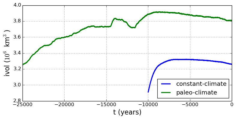
Fig. 8 Time series of modeled ice sheet volume ice_volume_glacierized from constant-climate (blue; ts_g20km_10ka_hy.nc) and paleo-climate (green; ts_g20km_25ka_paleo.nc) spinup runs. Note that the paleo-climate run started with the ice geometry at the end of the constant-climate run.

Another time-series comparison, of the variable ice_volume_glacierized_temperate, the total volume of temperate (at \(0^\circ C\)) ice, appears in Fig. 9. The paleo-climate run shows the cold period from \(\approx -25\) ka to \(\approx -12\) ka. Both constant-climate and paleo-climate runs then come into rough equilibrium in the holocene. The bootstrapping artifact, seen at the start of the constant-climate run, which disappears in less than 1000 years, is avoided in the paleo-climate run by starting with the constant-climate end-state. The reader is encouraged to examine the diagnostic files ts_g20km_25ka_paleo.nc and ex_g20km_25ka_paleo.nc to find more evidence of the (modeled) climate impact on the ice dynamics.

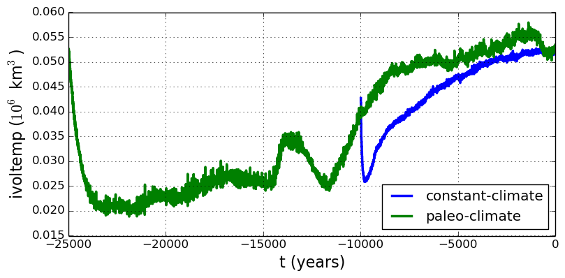
Fig. 9 Time series of temperate ice volume ice_volume_glacierized_temperate from constant-climate (blue; ts_g20km_10ka_hy.nc) and paleo-climate (green; ts_g20km_25ka_paleo.nc) spinup runs. The cold of the last ice age affects the fraction of temperate ice. Note different volume scale compared to that in Fig. 8; only about 1% of ice is temperate (by volume).

---

Previous

Up

Next