Computing ice age
By default, PISM does not compute the age of the ice because it does not directly impact ice flow when using the default flow laws. (But see Coupling to the age of the ice for SIA parameterizations that use it.)
Set age.enabled to turn it on. A 3D variable age will appear in output
files. It is read during model initialization if age.enabled is set and ignored
otherwise. If age.enabled is set and the variable age is absent in the
input file then the initial age is set to age.initial_value.
The first order upwinding method used to approximate the evolution of age is
diffusive, which leads to the loss of detail, especially near the base of the ice where
the variation of age with depth is more pronounced. Increasing vertical grid resolution
and using quadratic grid spacing (finer near the bed, coarser by a factor of
grid.lambda near the surface; see Spatial grid) would reduce the effect of
numerical diffusion but cannot eliminate it.
Isochronal layer tracing
To model closely-spaced isochrones PISM implements the isochronal layer tracing scheme described in [81] and [82]; see section 2.4 of the latter for details. This method uses a “Lagrangian” approximation in the vertical direction and a first-order upwinding method in horizontal directions. This eliminates numerical diffusion in the critical, vertical direction.
Note
This approximation assumes that the age of the ice increases monotonically with depth, so it cannot be used to model overturning folds [83] and plume formation [84].
Summary
Ice masses are interpreted as “stacks” of layers of varying thickness. Isochrones are represented by boundaries between these layers; the depth of an isochrone is the sum of thicknesses of all the layers above it (some may have zero thickness, e.g. in ablation and ice-free areas). The surface mass balance is applied to the topmost layer; if a layer is depleted by a negative mass balance, the remaining mass loss is used to reduce the thickness of the next layer below it. Similarly, the basal melt rate is applied to the bottom layer, then (if necessary) the one above it, etc. Within each layer mass is transported according to the horizontal components of the 3D ice velocity by sampling it at the depth of the middle of a layer. There is no mass transport between layers. A new layer is added to the top of the stack each time the simulation reaches a requested deposition time.
Set isochrones.deposition_times to enable this mechanism. This parameter takes
an argument in the format identical to output.spatial.times; see
Spatially-varying diagnostic quantities.
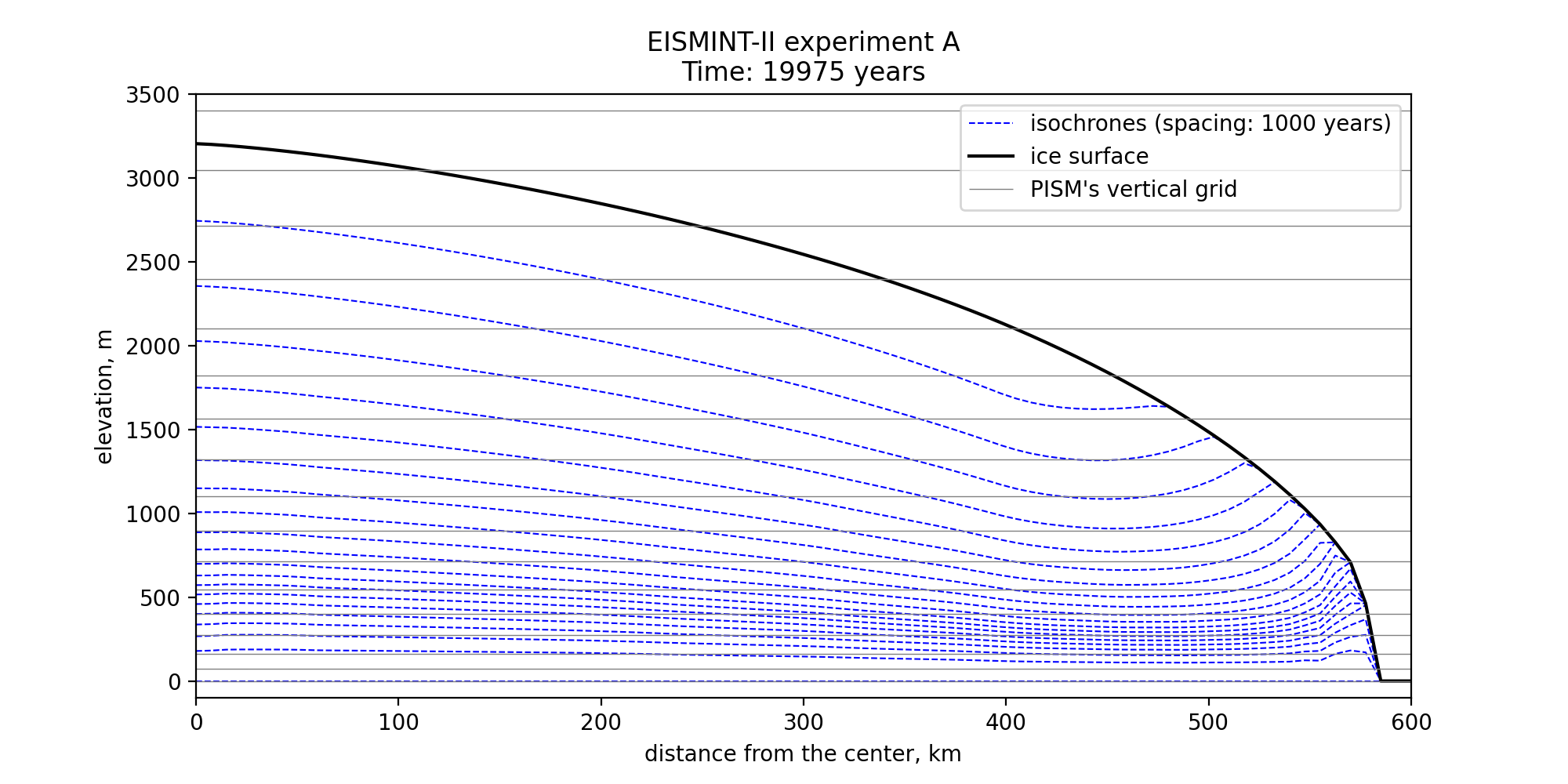
Fig. 22 Modeled isochrones after 20000 years from the start of the EISMINT-II
[85] experiment A. Note that many isochrones near the base are closer
than the vertical grid spacing. See the directory examples/isochrones in PISM’s
repository for scripts used to create this figure.
Model state
Layer thicknesses are saved to the variable isochronal_layer_thickness in an output
file. A subset of requested deposition times is saved to deposition_time. Since the
state of the model may be saved before a simulation reached all requested deposition times
some layers may not have been created. We use the time variable to identify
“active” layers: a layer is active if the model reached the corresponding deposition time.
Note
The time variable is used to interpret layer thicknesses and deposition times
read from an input file, so the current simulation has to be compatible with the one
that produced the model state used to initialize it.
If a simulation \(S_1\) is initialized using the output of a simulation \(S_0\), then \(S_1\) should start at the end of the time interval modeled by \(S_0\); also, \(S_0\) and \(S_1\) should use the same calendar and the reference date.
Bootstrapping
During bootstrapping deposition_time is set using isochrones.deposition_times.
We implement two ways of initializing isochronal_layer_thickness:
Default: interpret current ice thickness as one layer; apply surface mass balance to this layer until a new layer is added. This is appropriate when starting simulations from an ice-free initial state.
Divide current ice thickness equally into \(N\) layers (here \(N\) is set by
isochrones.bootstrapping.n_layers), then immediately add one more layer and apply SMB to it until a new layer is added. This may be appropriate when starting from an initial state with a significant ice thickness. In this case sampling ice velocity in the middle of the layer (halfway between the base and the surface) is likely give lower accuracy compared to sampling at \(N\) equally-spaced locations in each column of ice.
Regridding
Set -regrid_file foo.nc -regrid_vars isochronal_layer_thickness,... to read in
isochronal_layer_thickness from a file foo.nc using bilinear interpolation
instead of reading from input.file (without interpolation). Regridding layer
thicknesses bypasses bootstrapping heuristics.
Diagnostics
The isochronal tracing scheme provides one diagnostic: isochrone_depth (depth below
the surface for isochrones corresponding to all requested deposition times).
Note
It is not recommended to append diagnostics to the same file
(output.spatial.append) when re-starting a simulation. A restarted simulation
may not be able to write isochrone_depth and isochronal_layer_thickness
to the same file because of a difference in the number of deposition times handled by
the model in the two runs involved.
Parameters
Prefix: isochrones.
bootstrapping.n_layers(0) number of isochronal layers created during bootstrappingdeposition_timesList or a range of deposition times used to create isochronal layersmax_n_layers(100) maximum number of isochronal layers
| Previous | Up | Next |