MISMIP
This intercomparison addresses grounding line dynamics by considering an idealized one-dimensional stream-shelf system. In summary, a flowline ice stream and ice shelf system is modeled, the reversibility of grounding line movement under changes in the ice softness is tested, different sliding laws are tested, and the behavior of grounding lines on reverse-slope beds is tested. The intercomparison process is described at the website
Find a full text description there, along with the published report on the results [125]; that paper includes results from PISM version 0.1. These documents are essential reading for understanding MISMIP results generally, and for appreciating the brief discussion in this subsection.
PISM’s version of MISMIP includes an attached ice shelf even though modeling the shelf is theoretically unnecessary in the flow line case. The analysis in [127] shows that the only effect of an ice shelf, in the flow line case, is to transfer the force imbalance at the calving front directly to the ice column at the grounding line. Such an analysis does not apply to ice shelves with two horizontal dimensions; real ice shelves have “buttressing” and “side drag” and other forces not present in the flow line [128]. See the next subsection on MISMIP3d and the Ross ice shelf example in section An SSA flow model for the Ross Ice Shelf in Antarctica, among other examples.
We must adapt the usual 3D PISM model to two horizontal dimensions, i.e. to do flow-line
problems (see section Using PISM for flow-line modeling). The flow direction for MISMIP is
taken to be “\(x\)”. We periodize the cross-flow direction “\(y\)”, and use the minimum number
of points in the \(y\)-direction. This number turns out to be “-My 3”; fewer points than
this in the cross-flow direction confuses the finite difference scheme.
PISM can do MISMIP experiments with either of two applicable ice dynamics models. Model 1 is a pure SSA model; “category 2” in the MISMIP classification. Model 2 combines SIA and SSA velocities as described in [17]; “category 3” because it resolves “vertical” shear (i.e. using SIA flow).
There are many runs for a complete MISMIP intercomparison submission. Specifically, for a given model there are \(62\) runs for each grid choice, and three (suggested) grid choices, so a full suite is \(3 \times 62 = 186\) runs.
The coarsest grid (“mode 1”) has 12 km spacing. The finest grid, “mode 2” with 1.2 km spacing, accounts for all the compute time, however; in the MISMIP description it is 1500 grid spaces in the flow line direction (= 3001 grid points in PISM’s doubled computational domain). In between is “mode 3”, a mode interpretable by the intercomparison participant, and here we just use a 6 km grid.
The implementation of MISMIP in PISM conforms to the intercomparison description, but that document specifies
… we require that the rate of change of grounding line position be \(0.1\) m/a or less, while the rate of change of ice thickness at each grid point at which ice thickness is defined must be less than \(10^{-4}\) m/a…
as a standard for “steady state”. The scripts here do not implement this stopping criterion. However, we report enough information, in PISM output files with scalar and spatially-variable time-series, to compute a grounding line rate or the time at which the thickness rate of change drops below \(10^{-4}\) m/a.
See
examples/mismip/mismip2d/README.md
for usage of the scripts that run MISMIP experiments in PISM. For example, as described in
this README.md, the commands
./run.py -e 1a --mode=1 > experiment-1a-mode-1.sh
bash experiment-1a-mode-1.sh 2 >& out.1a-mode-1 &
./plot.py ABC1_1a_M1_A7.nc -p -o profileA7.png
first generate a bash script, then use it to do a run which takes about 20 minutes, and
then generate an image in .png format. Note that step 7 is in the middle of the
experiment. It is shown in Fig. 23 (left).
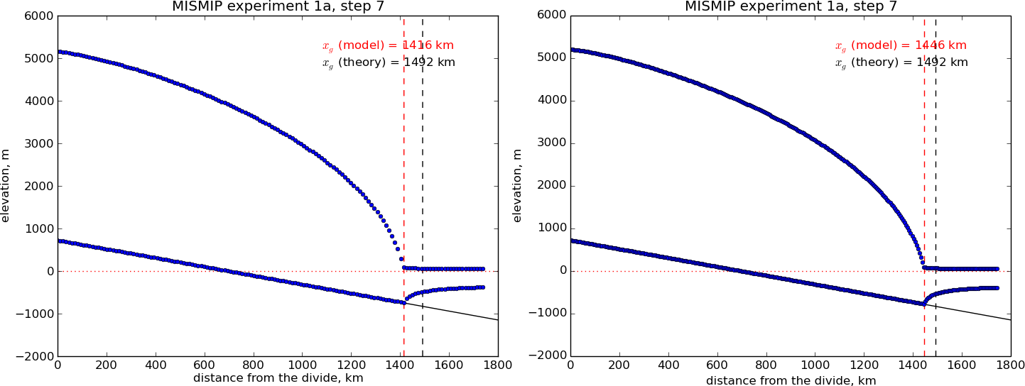
Fig. 23 A marine ice sheet profile in the MISMIP intercomparison; PISM model 1, experiment 1a, at step 7. Left: grid mode 1 (12 km grid). Right: grid mode 3 (6 km grid).
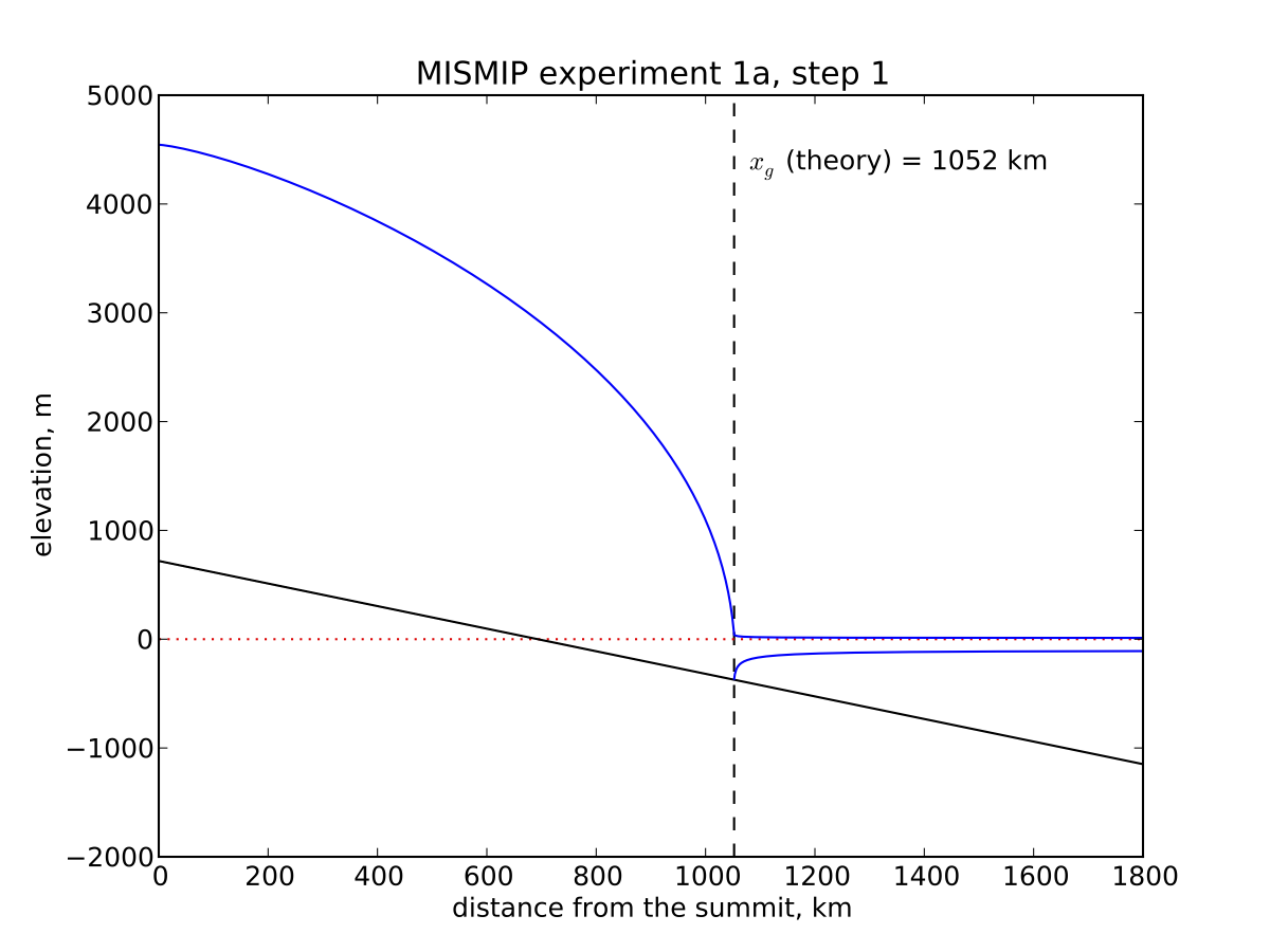
Fig. 24 Analytical profile for steady state of experiment 1a, step 1, from theory in [127]. This is a boundary layer asymptotic matching result, but not the exact solution to the equations.
The script MISMIP.py in examples/mismip/mismip2d has the ability to compute the
profile from the Schoof’s [127] asymptotic-matching boundary layer theory. This
script is a Python translation, using scipy and pylab, of the provided MATLAB
codes. For example,
python MISMIP.py -o mismip_analytic.png
produces a .png image file with Fig. 24. By default
run.py uses the asymptotic-matching thickness result from the [127] theory
to initialize the initial ice thickness, as allowed by the MISMIP specification.
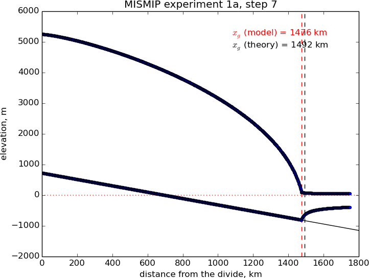
Fig. 25 Results from MISMIP grid mode 2, with 1.2 km spacing, for steady state of experiment 1a: profile at step 7 (compare Fig. 23).
Generally the PISM result does not put the grounding line in the same location as Schoof’s boundary layer theory, and at least at coarser resolutions the problem is with PISM’s numerical solution, not with Schoof’s semi-analytic theory. The result improves under grid refinement, however. Results from grid mode 3 with 6 km spacing, instead of 12 km in mode 1, are the right part of Fig. 23. The corresponding results from grid mode 2, with 1.2 km spacing, are in Figure Fig. 25. Note that the difference between the numerical grounding line location and the semi-analytical location has been reduced from 76 km for grid mode 1 to 16 km for grid mode 2 (a factor of about 5), by using a grid refinement from 12 km to 1.2 km (a factor of about 10).
| Previous | Up | Next |