An SIA flow model for a table-top laboratory experiment¶

Though there are additional complexities to the flow of real ice sheets, an ice sheet is a shear-thinning fluid with a free surface. PISM ought to be able to model such flows in some generality. We test that ability here by comparing PISM’s isothermal SIA numerical model to a laboratory observations of a 1% Xanthan gum suspension in water in a table-top, moving-margin experiment by R. Sayag and M. Worster [133], [134]. The “gum” fluid is more shear-thinning than ice, and it has much lower absolute viscosity values, but it has the same density. This flow has total mass \(\sim 1\) kg, compared to \(\sim 10^{18}\) kg for the Greenland ice sheet.

We compare our numerical results to the “constant-flux” experiment from [133]. Fig. 40 shows the experimental setup by reproducing Figures 2(c) and 2(d) from that reference. A pump pushes the translucent blue-dyed fluid through a round 8 mm hole in the middle of a clear table-top at a mass rate of about 3 gm/s. The downward-pointing camera, which produced the right-hand figure, allows measurement of the location of margin of the “ice cap”, and in particular of its radius. The measured radii data are the black dots in Fig. 41.

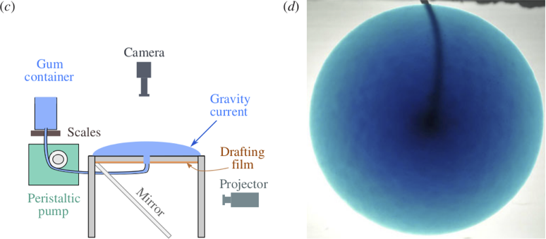
../../_images/labgumexperiment.png — Fig. 40 Reproduction of Figures 2(c) and 2(d) from [133]. Left: experimental apparatus used for “constant-flux release” experiment. Right: snapshot of constant-flux experiment (plan view), showing an axisymmetric front.¶

The closest glaciological analog would be an ice sheet on a flat bed fed by positive basal mass balance (i.e. “refreeze”) underneath the dome, but with zero mass balance elsewhere on the lower and upper surfaces. However, noting that the mass-continuity equation is vertically-integrated, we may model the input flux (mass balance) as arriving at the top of the ice sheet, to use PISM’s climate-input mechanisms. The flow though the input hole is simply modeled as constant across the hole, so the input “climate” uses -surface given with a field climatic_mass_balance, in the bootstrapping file, which is a positive constant in the hole and zero outside. While our replacement of flow into the base by mass balance at the top represents a very large change in the vertical component of the velocity field, we still see good agreement in the overall shape of the “ice sheet”, and specifically in the rate of margin advance.

Sayag & Worster estimate Glen exponent \(n = 5.9\) and a softness coefficient \(A = 9.7 \times 10^{-9}\,\text{Pa}^{-5.9}\,\text{s}^{-1}\) for the flow law of their gum suspension, using regression of laboratory measurements of the radius. (Compare PISM defaults \(n=3\) and \(A\approx 4\times 10^{-25}\,\text{Pa}^{-3}\,\text{s}^{-1}\) for ice.) Setting the Sayag & Worster values is one of several changes to the configuration parameters, compared to PISM ice sheet defaults, which are done in part by overriding parameters at run time by using the -config_override option. See examples/labgum/preprocess.py for the generation of a configuration .nc file with these settings.

To run the example on the default 10 mm grid, first do

./preprocess.py

and then do a run for 746 model seconds [133] on the 10 mm grid on a \(520\,\text{mm}\,\times 520\,\text{mm}\) square domain using 4 processors:

./rungum.sh 4 52 &> out.lab52 &

This run generates text file out.lab52, diagnostic files ts_lab52.nc and ex_lab52.nc, and final output lab52.nc. This run took about 5 minutes on a 2013 laptop, thus roughly real time! When it is done, you can compare the modeled radius to the experimental data:

./showradius.py -o r52.png -d constantflux3.txt ts_lab52.nc

You can also redo the whole thing on higher resolution grids (here: 5 and 2.5 mm), here using 6 MPI processes if the runs are done simultaneously, and when it is done after several hours, make a combined figure just like Fig. 41:

./preprocess.py -Mx 104 -o initlab104.nc
./preprocess.py -Mx 208 -o initlab208.nc
./rungum.sh 2 104 &> out.lab104 &
./rungum.sh 4 208 &> out.lab208 &
./showradius.py -o foo.png -d constantflux3.txt ts_lab*.nc

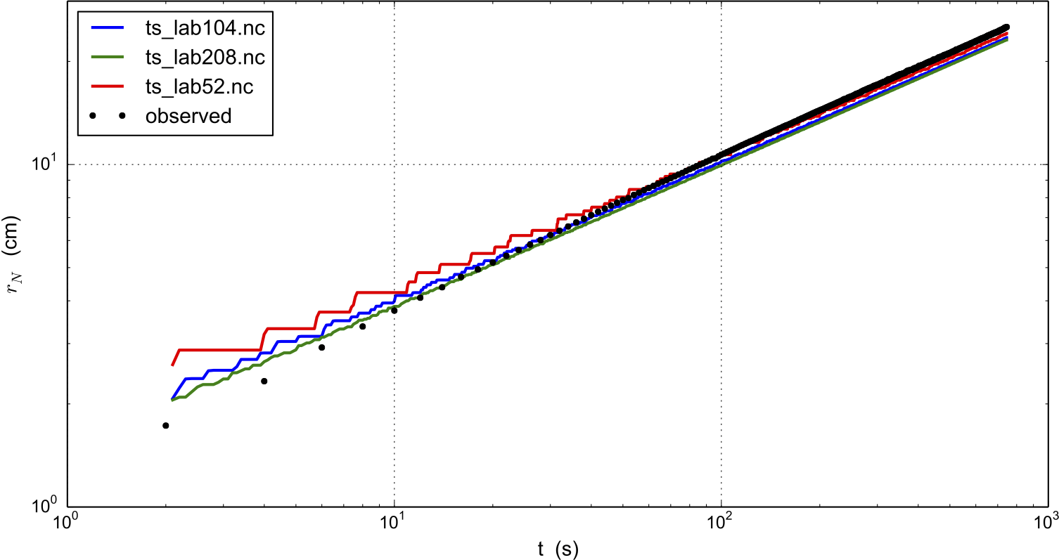
../../_images/labgumradius.png — Fig. 41 Radius \(r_N(t)\) for runs with 10 mm (`ts_lab52.nc`), 5 mm (`ts_lab104.nc`), and 2.5 mm (`ts_lab208.nc`) grids, compared to observations from Sayag & Worster’s [133] table-top “ice cap” (gravity current) made from a 1% Xanthan gum suspension, as shown in Figure Fig. 40.¶

We see that on the coarsest grid the modeled volume has “steps” because the margin advances discretely. Note we are computing the radius by first computing the fluid-covered area \(a\) on the cartesian grid, and then using \(a=\pi r^2\) to compute the radius.

Results are better on finer grids, especially at small times, because the input hole has radius of only 8 mm. Furthermore this “ice cap” has radius comparable to the hole for the first few model seconds. The early evolution is thus distinctly non-shallow, but we see that increasing the model resolution reduces most of the observation-model difference. In fact there is little need for “higher-order” stresses because the exact similarity solution of the shallow continuum equations, used by Sayag & Worster, closely-fits the data even for small radius and time (see [133], Figure 4).

In any case, the large-time observations are very closely-fit by the numerical results at all grid resolutions. We have used the Glen-law parameters \(n,A\) as calculated by Sayag & Worster, but one could do parameter-fitting to get the “best” values if desired. In particular, roughly speaking, \(n\) controls the slope of the results in Fig. 41 and \(A\) controls their vertical displacement.