On the vertical coordinate in PISM, and a critical change of variable

In PISM all fields in the ice, including enthalpy, age, velocity, and so on, evolve within an ice fluid domain of changing geometry. See Fig. 48. In particular, the upper and lower surfaces of the ice fluid move with respect to the geoid.

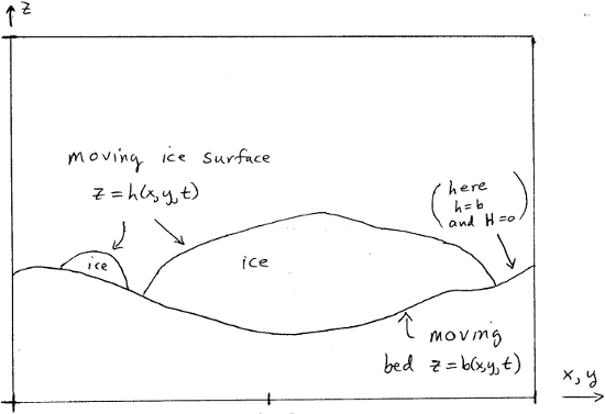
Fig. 48 The ice fluid domain evolves, with both the upper and lower surfaces in motion with respect to the geoid.

Note

FIXME: This figure should show the floating case too.

The \((x,y,z)\) coordinates in Fig. 48 are supposed to be from an orthogonal coordinate system with \(z\) in the direction anti-parallel to gravity, so this is a flat-earth approximation. In practice, the data inputs to PISM are in some particular projection, of course.

We make a change of the independent variable \(z\) which simplifies how PISM deals with the changing geometry of the ice, especially in the cases of a non-flat or moving bed. We replace the vertical coordinate relative to the geoid with the vertical coordinate relative to the base of the ice. Let

\[\begin{split}s = \begin{cases} z - b(x,y,t), & \text{ice is grounded}, \\ z - \frac{\rho_i}{\rho_o} H(x,y,t), & \text{ice is floating;} \end{cases}\end{split}\]

where \(H = h - b\) is the ice thickness and \(\rho_i, \rho_o\) are densities of ice and ocean, respectively.

Now we make the change of variables

\[(x,y,z,t) \mapsto (x,y,s,t)\]

throughout the PISM code. This replaces \(z=b\) by \(s=0\) as the equation of the base surface of the ice. The ice fluid domain in the new coordinates only has a free upper surface as shown in Fig. 49.

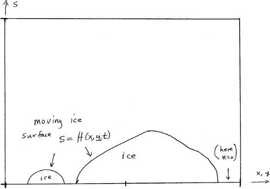
Fig. 49 In (x,y,s) space the ice fluid domain only has an upper surface which moves, \(s=H(x,y,t)\). Compare to Fig. 48.

Note

FIXME: This figure should show the floating case too, and bedrock.”

In PISM the computational domain (region)

\[\mathcal{R}=\left\{(x,y,s)\big| -L_x\le x \le L_x, -L_y\le y \le L_y, -Lb_z \le s \le L_z\right\}\]

is divided into a three-dimensional grid. See IceGrid.

The change of variable \(z\to s\) used here is not the [171] change of variable \(\tilde s=(z-b)/H\) . That change causes the conservation of energy equation to become singular at the boundaries of the ice sheet. Specifically, the Jenssen change replaces the vertical conduction term by a manifestly-singular term at ice sheet margins where \(H\to 0\), because

\[\frac{\partial^2 E}{\partial z^2} = \frac{1}{H^2} \frac{\partial^2 E}{\partial \tilde s^2}.\]

A singular coefficient of this type can be assumed to affect the stability of all time-stepping schemes. The current change \(s=z-b\) has no such singularizing effect though the change does result in added advection terms in the conservation of energy equation, which we now address. See BOMBPROOF, PISM’s numerical scheme for conservation of energy for more general considerations about the conservation of energy equation.

The new coordinates \((x,y,s)\) are not orthogonal.

Recall that if \(f=f(x,y,z,t)\) is a function written in the old variables and if \(\tilde f(x,y,s,t)=f(x,y,z(x,y,s,t),t)\) is the “same” function written in the new variables, equivalently \(f(x,y,z,t)=\tilde f(x,y,s(x,y,z,t),t)\) , then

\[\diff{f}{x} = \diff{\tilde f}{x} + \diff{\tilde f}{s} \diff{s}{x} = \diff{\tilde f}{x} - \diff{\tilde f}{s} \diff{b}{x}.\]

Similarly,

\[\diff{f}{y} = \diff{\tilde f}{y} - \diff{\tilde f}{s} \diff{b}{y},\]

\[\diff{f}{t} = \diff{\tilde f}{t} - \diff{\tilde f}{s} \diff{b}{t}.\]

On the other hand,

\[\diff{f}{z} = \diff{\tilde f}{s}.\]

The following table records some important changes to formulae related to conservation of energy:

\[\begin{split}\begin{array}{ll} \textbf{old} & \textbf{new} \\ P=\rho g(h-z) & P=\rho g(H-s) \\ \diff{E}{t} & \diff{E}{t}-\diff{E}{s}\diff{b}{t} \\ \nabla E & \nabla E- \diff{E}{s}\nabla b \\ \rho_i\left(\diff{E}{t}+\mathbf{U}\cdot\nabla E + w\diff{E}{z}\right)=\frac{k_i}{c_i} \frac{\partial^2 E}{\partial z^2} + Q & \rho_i\left(\diff{E}{t} + \mathbf{U}\cdot\nabla E + \left(w-\diff{b}{t}-\mathbf{U}\cdot\nabla b\right)\diff{E}{s}\right) = \frac{k_i}{c_i} \frac{\partial^2 E}{\partial s^2} + Q \end{array}\end{split}\]

Note \(E\) is the ice enthalpy and \(T\) is the ice temperature (which is a function of the enthalpy; see EnthalpyConverter), \(P\) is the ice pressure (assumed hydrostatic), \(\mathbf{U}\) is the depth-dependent horizontal velocity, and \(Q\) is the strain-heating term.

Now the vertical velocity is computed by StressBalance::compute_vertical_velocity(...). In the old coordinates \((x,y,z,t)\) it has this formula:

\[w(z) = -\int_b^z \diff{u}{x}(z') + \diff{v}{y}(z')\,dz' + \diff{b}{t} + \mathbf{U}_b \cdot \nabla b - S.\]

Here \(S\) is the basal melt rate, positive when ice is being melted. We have used the basal kinematical equation and integrated the incompressibility statement

\[\diff{u}{x} + \diff{v}{y} + \diff{w}{z} = 0.\]

In the new coordinates we have

\[w(s) = -\int_0^s \diff{u}{x}(s') + \diff{v}{y}(s')\,ds' + \mathbf{U}(s) \cdot \nabla b + \diff{b}{t} - S.\]

(Note that the term \(\mathbf{U}(s) \cdot \nabla b\) evaluates the horizontal velocity at level \(s\) and not at the base.)

Let

\[\tilde w(x,y,s,t) = w(s) - \diff{b}{t}-\mathbf{U}(s)\cdot\nabla b.\]

This quantity is the vertical velocity of the ice relative to the location on the bed immediately below it. In particular, \(\tilde w=0\) for a slab sliding down a non-moving inclined plane at constant horizontal velocity, if there is no basal melt rate. Also, \(\tilde w(s=0)\) is nonzero only if there is basal melting or freeze-on, i.e. when \(S\ne 0\). Within PISM, \(\tilde w\) is written with name \(wvel_rel\) into an input file. Comparing the last two equations, we see how StressBalance::compute_vertical_velocity(...) computes \(\tilde w\) :

\[\tilde w(s) = -\int_0^s \diff{u}{x}(s') + \diff{v}{y}(s')\,ds' - S.\]

The conservation of energy equation is now, in the new coordinate \(s\) and newly-defined relative vertical velocity,

\[\rho_i \left(\diff{E}{t} + \mathbf{U}\cdot\nabla E + \tilde w \diff{E}{s}\right) = \frac{k_i}{c_i} \frac{\partial^2 E}{\partial s^2} + Q.\]

Thus it looks just like the conservation of energy equation in the original vertical velocity \(z\). This is the form of the equation solved by EnthalpyModel using enthSystemCtx::solve().

Under option -o_size big, all of these vertical velocity fields are available as fields in the output NetCDF file. The vertical velocity relative to the geoid, as a three-dimensional field, is written as the diagnostic variable wvel. This is the “actual” vertical velocity \(w = \tilde w + \diff{b}{t} + \mathbf{U}(s)\cdot\nabla b\) . Its surface value is written as wvelsurf, and its basal value as wvelbase. The relative vertical velocity \(\tilde w\) is written to the NetCDF output file as wvel_rel.

---

Previous

Up

Next