Surface mass and energy process model components ¶

Contents

Surface mass and energy process model components

The “invisible” model ¶

Options: -surface simple
Variables: none
C++ class: pism::surface::Simple

This is the simplest “surface model” available in PISM, enabled using -surface simple. Its job is to re-interpret precipitation as climatic mass balance, and to re-interpret mean annual near-surface (2m) air temperature as the temperature of the ice at the depth at which firn processes cease to change the temperature of the ice. (I.e. the temperature below the firn.) This implies that there is no melt. Though primitive, this model component may be desired in cold environments (e.g. East Antarctic ice sheet) in which melt is negligible and heat from firn processes is ignored.

Reading top-surface boundary conditions from a file ¶

Options: -surface given
Variables: ice_surface_temp, climatic_mass_balance \(kg / (m^{2} s)\)
C++ class: pism::surface::Given

Note

This is the default choice.

This model component was created to force PISM with sampled (possibly periodic) climate data by reading ice upper surface boundary conditions from a file. These fields are provided directly to the ice dynamics code (see Climate inputs, and their interface with ice dynamics for details).

PISM will stop if variables ice_surface_temp (ice temperature at the ice surface but below firn) and climatic_mass_balance (top surface mass flux into the ice) are not present in the input file.

A file foo.nc used with -surface given -surface_given_file foo.nc may contain several records. If this file contains one record (i.e. fields corresponding to one time value only), provided forcing data is interpreted as time-independent. Variables time and time_bnds should specify model times corresponding to individual records.

For example, to use monthly periodic forcing with a period of 1 year starting at the beginning of \(1980\) (let’s use the \(360\)-day calendar for simplicity), create a file (say, “foo.nc”) with 12 records. The time variable may contain \(15, 45, 75, \dots, 345\) (mid-month for all \(12\) months) and have the units of “days since 1980-1-1”. (It is best to avoid units of “months” and “years” because their meanings depend on the calendar.) Next, add the time_bounds variable for the time dimension with the values \(0, 30, 30, 60, \dots\) specifying times corresponding to beginnings and ends of records for each month and set the time:bounds attribute accordingly. Now run

pismr -surface given -surface_given_file foo.nc -surface.given.periodic

See Using time-dependent forcing for more information.

Note

This surface model ignores the atmosphere model selection made using the option -atmosphere.
PISM can handle files with virtually any number of records: it will read and store in memory at most input.forcing.buffer_size records at any given time (default: 60, or 5 years’ worth of monthly fields).
when preparing a file for use with this model, it is best to use the t,y,x variable storage order: files using this order can be read in faster than ones using the t,x,y order, for reasons explained in the User’s Manual.

To change the storage order in a NetCDF file, use ncpdq:
```
ncpdq -a t,y,x input.nc output.nc
```
will copy data from input.nc into output.nc, changing the storage order to t,y,x at the same time.

Parameters

Prefix: surface.given.

file Name of the file containing climate forcing fields.
periodic (no) If true, interpret forcing data as periodic in time
smb_max (91000 kg m-2 year-1) Maximum climatic mass balance value (used to check input data). Corresponds to 100 m/year ice equivalent.

Elevation-dependent temperature and mass balance ¶

Options: -surface elevation
Variables: none
C++ class: pism::surface::Elevation

This surface model component parameterizes the ice surface temperature \(T_{h}\) = ice_surface_temp and the mass balance \(m\) = climatic_mass_balance as piecewise-linear functions of surface elevation \(h\).

The option -ice_surface_temp (list of 4 numbers) determines the surface temperature using the 4 parameters \(\T{min}\), \(\T{max}\), \(\h{min}\), \(\h{max}\). Let

\[\diff{T}{h} = (\T{max} - \T{min}) / (\h{max} - \h{min})\]

be the temperature gradient. Then

\[\begin{split}T(x,y) = \begin{cases} \T{min}, & h(x,y) \le \h{min}, \\ \T{min} + \diff{T}{h} \, (h(x,y) - \h{min}), & \h{min} < h(x,y) < \h{max}, \\ \T{max}, & \h{max} \le h(x,y). \end{cases}\end{split}\]

The option -climatic_mass_balance (list of 5 numbers) determines the surface mass balance using the 5 parameters \(\m{min}\), \(\m{max}\), \(\h{min}\), \(\h{ELA}\), \(\h{max}\). Let

\[\diff{\m{abl}}{h} = -\m{min} / (\ELA - \h{min})\]

and

\[\diff{\m{acl}}{h} = \m{max} / (\h{max} - \ELA)\]

be the mass balance gradient in the ablation and in the accumulation area, respectively. Then

\[\begin{split}m(x,y) = \begin{cases} \m{min}, & h(x,y) \le \h{min}, \\ \diff{\m{abl}}{h} \, (h(x,y) - \ELA), & \h{min} < h(x,y) \le \ELA, \\ \diff{\m{acl}}{h} \, (h(x,y) - \ELA), & \ELA < h(x,y) \le \h{max}, \\ \m{max}, & \h{max} < h(x,y). \end{cases}\end{split}\]

The option -climatic_mass_balance_limits (list of 2 numbers) limits the mass balance below \(\h{min}\) to \(\ms{min}\) and above \(\h{max}\) to \(\ms{max}\), thus

\[\begin{split}m(x,y) = \begin{cases} m^{*}_{\text{min}}, & h(x,y) \le \h{min}, \\ \diff{\m{abl}}{h} \, (h(x,y) - \ELA), & \h{min} < h(x,y) \le \ELA, \\ \diff{\m{acl}}{h} \, (h(x,y) - \ELA), & \ELA < h(x,y) \le \h{max}, \\ m^{*}_{\text{max}}, & \h{max} < h(x,y). \end{cases}\end{split}\]

Note: this surface model ignores the atmosphere model selection made using the -atmosphere option.

Temperature-index scheme ¶

Options: -surface pdd
Variables: air_temp_sd, snow_depth
C++ class: pism::surface::TemperatureIndex

The default PDD model used by PISM, turned on by option -surface pdd, is based on [18] and EISMINT-Greenland intercomparison (see [7]).

Our model computes the solid (snow) precipitation rate using the air temperature threshold with a linear transition. All precipitation during periods with air temperatures above surface.pdd.air_temp_all_precip_as_rain (default of \(2^\circ C\)) is interpreted as rain; all precipitation during periods with air temperatures below surface.pdd.air_temp_all_precip_as_snow (default of \(0^\circ C\)) is interpreted as snow.

For long-term simulations, a PDD model generally uses an idealized seasonal temperature cycle. “White noise” is added to this cycle to simulate additional daily variability associated to the vagaries of weather. This additional random variation is quite significant, as the seasonal cycle may never reach the melting point but that point may be reached with some probability, in the presence of the daily variability, and thus melt may occur. Concretely, a normally-distributed, mean zero random temperature increment is added to the seasonal cycle. There is no assumed spatial correlation of daily variability. The standard deviation of the daily variability is controlled by configuration parameters with the prefix surface.pdd.std_dev.:

file The name of the file to read air_temp_sd (standard deviation of air temperature) from.
lapse_lat_base (72 degree_north) standard deviationis is a function of latitude, with value surface.pdd.std_dev.value at this latitude; this value is only active if surface.pdd.std_dev.lapse_lat_rate is nonzero
lapse_lat_rate (0 Kelvin / degree_north) standard deviation is a function of latitude, with rate of change with respect to latitude given by this constant
param_a (-0.15) Parameter \(a\) in \(\Sigma = aT + b\), with \(T\) in degrees C. Used only if surface.pdd.std_dev.use_param is set to yes.
param_b (0.66 Kelvin) Parameter \(b\) in \(\Sigma = aT + b\), with \(T\) in degrees C. Used only if surface.pdd.std_dev.use_param is set to yes.
periodic (no) If true, interpret air_temp_sd read from surface.pdd.std_dev.file as periodic in time
use_param (no) Parameterize standard deviation as a linear function of air temperature over ice-covered grid cells. The region of application is controlled by geometry.ice_free_thickness_standard.
value (5 Kelvin) standard deviation of daily temp variation; = EISMINT-Greenland value [7]

A file foo.nc used with -surface pdd -pdd_sd_file foo.nc should contain standard deviation of near-surface air temperature in variable air_temp_sd, and the corresponding time coordinate in variable time. If -pdd_sd_file is not set, PISM uses a constant value for standard deviation, which is set by the configuration parameter surface.pdd.std_dev.value. The default value is \(5.0\) degrees [7]. However, this approach is not recommended as it induces significant errors in modeled surface mass balance in both ice-covered and ice-free regions [19], [20].

Over ice-covered grid cells, daily variability can also be parameterized as a linear function of near-surface air temperature \(\sigma = a \cdot T + b\) using the surface.pdd.std_dev.use_param configuration flag, and the corresponding parameters surface.pdd.std_dev.param_a and surface.pdd.std_dev.param_b. This parametrization replaces prescribed standard deviation values over glacierized grid cells as defined by the mask variable (see geometry.ice_free_thickness_standard). Default values for the slope \(a\) and intercept \(b\) were derived from the ERA-40 reanalysis over the Greenland ice sheet [21].

The number of positive degree days is computed as the magnitude of the temperature excursion above \(0\!\phantom{|}^\circ \text{C}\) multiplied by the duration (in days) when it is above zero.

In PISM there are two methods for computing the number of positive degree days. The first computes only the expected value, by the method described in [18]. This is the default when a PDD is chosen (i.e. option -surface pdd). The second is a Monte Carlo simulation of the white noise itself, chosen by adding the option -pdd_method random_process. This Monte Carlo simulation adds the same daily variation at every point, though the seasonal cycle is (generally) location dependent. If repeatable randomness is desired use -pdd_method repeatable_random_process instead.

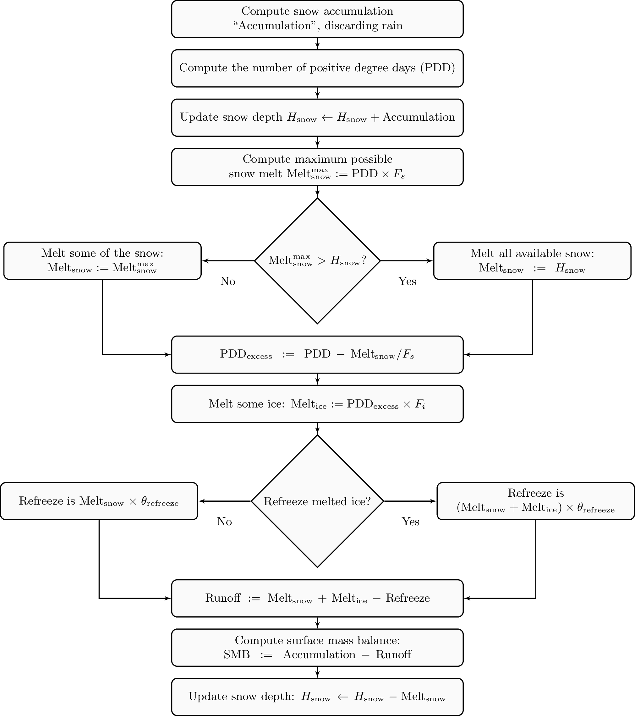
Fig. 46 PISM’s positive degree day model. \(F_s\) and \(F_i\) are PDD factors for snow and ice, respectively; \(\theta_{\text{refreeze}}\) is the refreeze fraction.¶

By default, the computation summarized in Fig. 46 is performed every week. (This frequency is controlled by the parameter surface.pdd.max_evals_per_year.) To compute mass balance during each week-long time-step, PISM keeps track of the current snow depth (using units of ice-equivalent thickness). This is necessary to determine if melt should be computed using the degree day factor for snow (surface.pdd.factor_snow) or the corresponding factor for ice (surface.pdd.factor_ice).

A fraction of the melt controlled by the configuration parameter surface.pdd.refreeze (\(\theta_{\text{refreeze}}\) in Fig. 46, default: \(0.6\)) refreezes. The user can select whether melted ice should be allowed to refreeze using the configuration flag surface.pdd.refreeze_ice_melt.

Since PISM does not have a principled firn model, the snow depth is set to zero at the beginning of the balance year. See surface.pdd.balance_year_start_day. Default is \(274\), corresponding to October 1^st.

Our PDD implementation is meant to be used with an atmosphere model implementing a cosine yearly cycle such as searise_greenland (section SeaRISE-Greenland), but it is not restricted to parameterizations like these.

This code also implements latitude- and mean July temperature dependent ice and snow factors using formulas (6) and (7) in [1]; set -pdd_fausto to enable. The default standard deviation of the daily variability (option -pdd_std_dev) is 2.53 degrees when -pdd_fausto is set [1]. See also configuration parameters with the prefix surface.pdd.fausto.:

T_c (272.15 Kelvin) = -1 + 273.15; for formula (6) in [1]
T_w (283.15 Kelvin) = 10 + 273.15; for formula (6) in [1]
beta_ice_c (0.015 meter / (Kelvin day)) water-equivalent thickness; for formula (6) in [1]
beta_ice_w (0.007 meter / (Kelvin day)) water-equivalent thickness; for formula (6) in [1]
beta_snow_c (0.003 meter / (Kelvin day)) water-equivalent thickness; for formula (6) in [1]
beta_snow_w (0.003 meter / (Kelvin day)) water-equivalent thickness; for formula (6) in [1]
enabled (false) Set PDD parameters using formulas (6) and (7) in [1]
latitude_beta_w (72 degree_north) latitude below which to use warm case, in formula (6) in [1]

Note that when used with periodic climate data (air temperature and precipitation) that is read from a file (see section Reading boundary conditions from a file), use of time_stepping.hit_multiples is recommended: set it to the length of the climate data period in years.

This model provides the following scalar:

surface_accumulation_rate
surface_melt_rate
surface_runoff_rate

and these 2D diagnostic quantities (averaged over reporting intervals; positive flux corresponds to ice gain):

surface_accumulation_flux
surface_melt_flux
surface_runoff_flux

This makes it easy to compare the surface mass balance computed by the model to its individual components:

SMB = surface_accumulation_flux - surface_runoff_flux

Parameters

Prefix: surface.pdd..

air_temp_all_precip_as_rain (275.15 Kelvin) threshold temperature above which all precipitation is rain; must exceed surface.pdd.air_temp_all_precip_as_snow to avoid division by zero, because difference is in a denominator
air_temp_all_precip_as_snow (273.15 Kelvin) threshold temperature below which all precipitation is snow
balance_year_start_day (274 ordinal day number) day of year for October 1st, beginning of the balance year in northern latitudes.
factor_ice (0.00879121 meter / (Kelvin day)) EISMINT-Greenland value [7]; = (8 mm liquid-water-equivalent) / (pos degree day)
factor_snow (0.0032967 meter / (Kelvin day)) EISMINT-Greenland value [7]; = (3 mm liquid-water-equivalent) / (pos degree day)
fausto.T_c (272.15 Kelvin) = -1 + 273.15; for formula (6) in [1]
fausto.T_w (283.15 Kelvin) = 10 + 273.15; for formula (6) in [1]
fausto.beta_ice_c (0.015 meter / (Kelvin day)) water-equivalent thickness; for formula (6) in [1]
fausto.beta_ice_w (0.007 meter / (Kelvin day)) water-equivalent thickness; for formula (6) in [1]
fausto.beta_snow_c (0.003 meter / (Kelvin day)) water-equivalent thickness; for formula (6) in [1]
fausto.beta_snow_w (0.003 meter / (Kelvin day)) water-equivalent thickness; for formula (6) in [1]
fausto.enabled (false) Set PDD parameters using formulas (6) and (7) in [1]
fausto.latitude_beta_w (72 degree_north) latitude below which to use warm case, in formula (6) in [1]
firn_compaction_to_accumulation_ratio (0.75) How much firn as a fraction of accumulation is turned into ice
firn_depth_file The name of the file to read the firn_depth from.
interpret_precip_as_snow (no) Interpret precipitation as snow fall.
max_evals_per_year (52) maximum number of times the PDD scheme will ask for air temperature and precipitation to build location-dependent time series for computing (expected) number of positive degree days and snow accumulation; the default means the PDD uses weekly samples of the annual cycle; see also surface.pdd.std_dev.value
method (expectation_integral) PDD implementation method
positive_threshold_temp (273.15 Kelvin) temperature used to determine meaning of “positive” degree day
refreeze (0.6) EISMINT-Greenland value [7]
refreeze_ice_melt (yes) If set to “yes”, refreeze surface.pdd.refreeze fraction of melted ice, otherwise all of the melted ice runs off.
std_dev.file The name of the file to read air_temp_sd (standard deviation of air temperature) from.
std_dev.lapse_lat_base (72 degree_north) standard deviationis is a function of latitude, with value surface.pdd.std_dev.value at this latitude; this value is only active if surface.pdd.std_dev.lapse_lat_rate is nonzero
std_dev.lapse_lat_rate (0 Kelvin / degree_north) standard deviation is a function of latitude, with rate of change with respect to latitude given by this constant
std_dev.param_a (-0.15) Parameter \(a\) in \(\Sigma = aT + b\), with \(T\) in degrees C. Used only if surface.pdd.std_dev.use_param is set to yes.
std_dev.param_b (0.66 Kelvin) Parameter \(b\) in \(\Sigma = aT + b\), with \(T\) in degrees C. Used only if surface.pdd.std_dev.use_param is set to yes.
std_dev.periodic (no) If true, interpret air_temp_sd read from surface.pdd.std_dev.file as periodic in time
std_dev.use_param (no) Parameterize standard deviation as a linear function of air temperature over ice-covered grid cells. The region of application is controlled by geometry.ice_free_thickness_standard.
std_dev.value (5 Kelvin) standard deviation of daily temp variation; = EISMINT-Greenland value [7]

PIK ¶

Options: -surface pik
Variables: climatic_mass_balance \(kg / (m^{2} s)\), lat (latitude), (degrees north)
C++ class: pism::surface::PIK

This surface model component implements the setup used in [3]. The climatic_mass_balance is read from an input (-i) file; the ice surface temperature is computed as a function of latitude (variable lat) and surface elevation (dynamically updated by PISM). See equation (1) in [3].

Scalar temperature offsets ¶

Options: -surface ...,delta_T
Variables: delta_T
C++ class: pism::surface::Delta_T

The time-dependent scalar offsets delta_T are added to ice_surface_temp computed by a surface model.

Please make sure that delta_T has the units of “Kelvin”.

This modifier is identical to the corresponding atmosphere modifier, but applies offsets at a different stage in the computation of top-surface boundary conditions needed by the ice dynamics core.

Parameters

Prefix: surface.delta_T.

file Name of the file containing temperature offsets.
periodic (no) If true, interpret forcing data as periodic in time

Adjustments using modeled change in surface elevation ¶

Options: -surface ...,elevation_change
Variables: surface_altitude (CF standard name),
C++ class: pism::surface::LapseRates

The elevation_change modifier adjusts ice-surface temperature and surface mass balance using modeled changes in surface elevation relative to a reference elevation read from a file.

The surface temperature is modified using an elevation lapse rate \(\gamma_T =\) surface.elevation_change.temperature_lapse_rate. Here

\[\gamma_T = -\frac{dT}{dz}.\]

Two methods of adjusting the SMB are available:

Scaling using an exponential factor

\[\mathrm{SMB} = \mathrm{SMB_{input}} \cdot \exp(C \cdot \Delta T),\]

where \(C =\) surface.elevation_change.smb.exp_factor and \(\Delta T\) is the temperature difference produced by applying surface.elevation_change.temperature_lapse_rate.

This mechanisms increases the SMB by \(100(\exp(C) - 1)\) percent for each degree of temperature increase.

To use this method, set -smb_adjustment scale.
Elevation lapse rate for the SMB

\[\mathrm{SMB} = \mathrm{SMB_{input}} - \Delta h \cdot \gamma_M,\]

where \(\gamma_M =\) surface.elevation_change.smb.lapse_rate and \(\Delta h\) is the difference between modeled and reference surface elevations.

To use this method, set -smb_adjustment shift.

Parameters

Prefix: surface.elevation_change..

file Name of the file containing the reference surface elevation field (variable usurf).
periodic (no) If true, interpret forcing data as periodic in time
smb.exp_factor (0 Kelvin-1) Exponential for the surface mass balance.
smb.lapse_rate (0 (m / year) / km) Lapse rate for the surface mass balance.
smb.method (shift) Choose the SMB adjustment method. scale: use temperature-change-dependent scaling factor. shift: use the SMB lapse rate.
temperature_lapse_rate (0 K / km) Lapse rate for the temperature at the top of the ice.

Mass flux adjustment ¶

Options: -surface ...,forcing
Variables: thk (ice thickness), ftt_mask (mask of zeros and ones; 1 where surface mass flux is adjusted and 0 elsewhere)
C++ class: pism::surface::ForceThickness

The forcing modifier implements a surface mass balance adjustment mechanism which forces the thickness of grounded ice to a target thickness distribution at the end of the run. The idea behind this mechanism is that spinup of ice sheet models frequently requires the surface elevation to come close to measured values at the end of a run. A simpler alternative to accomplish this, namely option -no_mass, represents an unmodeled, frequently large, violation of the mass continuity equation.

In more detail, let \(H_{\text{tar}}\) be the target thickness. Let \(H\) be the time-dependent model thickness. The surface model component described here produces the term \(M\) in the mass continuity equation:

\[\frac{\partial H}{\partial t} = M - S - \nabla\cdot \mathbf{q}.\]

(Other details of this equation do not concern us here.) The forcing modifier causes \(M\) to be adjusted by a multiple of the difference between the target thickness and the current thickness,

\[\Delta M = \alpha (H_{\text{tar}} - H)\]

where \(\alpha>0\). We are adding mass (\(\Delta M>0\)) where \(H_{\text{tar}} > H\) and ablating where \(H_{\text{tar}} < H\).

Option -force_to_thickness_file identifies the file containing the target ice thickness field thk and the mask ftt_mask. A basic run modifying surface model given would look like

pismr -i foo.nc -surface given,forcing -force_to_thickness_file bar.nc

In this case foo.nc contains fields climatic_mass_balance and ice_surface_temp, as normal for -surface given, and bar.nc contains fields thk which will serve as the target thickness and ftt_mask which defines the map plane area where this adjustment is applied. Option -force_to_thickness_alpha adjusts the value of \(\alpha\), which has a default value specified in the Configuration parameters.

In addition to this one can specify a multiplicative factor \(C\) used in areas where the target thickness field has less than -force_to_thickness_ice_free_thickness_threshold meters of ice; \(\alpha_{\text{ice free}} = C \times \alpha\). Use the -force_to_thickness_ice_free_alpha_factor option to set \(C\).

Using climate data anomalies ¶

Options: -surface ...,anomaly
Variables: ice_surface_temp_anomaly, climatic_mass_balance_anomaly \(kg / (m^{2} s)\)
C++ class: pism::surface::Anomaly

This modifier implements a spatially-variable version of -surface ...,delta_T which also applies time-dependent climatic mass balance anomalies.

See also -atmosphere ...,anomaly (section Using climate data anomalies), which is similar but applies anomalies at the atmosphere level.

Parameters

Prefix: surface.anomaly.

file Name of the file containing climate forcing fields.
periodic (no) If true, interpret forcing data as periodic in time

The caching modifier ¶

Options: -surface ...,cache
C++ class: pism::surface::Cache
See also: The caching modifier

This modifier skips surface model updates, so that a surface model is called no more than every surface.cache.update_interval 365-day “years”. A time-step of \(1\) year is used every time a surface model is updated.

This is useful in cases when inter-annual climate variability is important, but one year differs little from the next. (Coarse-grid paleo-climate runs, for example.)

Parameters

Prefix: surface.cache.

update_interval (10 365days) Update interval (in 365-day years) for the -surface cache modifier.

Preventing grounding line retreat ¶

Options: -surface ...,no_gl_retreat
C++ class: pism::surface::NoGLRetreat

This modifier adjust the surface mass balance to prevent the retreat of the grounding line. See Till friction angle optimization for an application.

Note

This modifier adds mass in violation of mass conservation. Save the diagnostic no_gl_retreat_smb_adjustment to get an idea about the amount added. Note, though, that this is an imperfect measure: it includes mass added to maintain non-negativity of ice thickness.
We assume that the sea level and the bed elevation remain constant throughout the simulation.
This does not prevent grounding line retreat caused by the thinning of the ice due to the melt at the base. Set geometry.update.use_basal_melt_rate to “false” to ensure that basal melt has no effect on the position of the grounding line