Testing if forcing data is used correctly
It is very important to ensure that selected forcing options produce the result you expect: we find that the ice sheet response is very sensitive to provided climate forcing, especially in short-scale simulations.
This section describes how to use PISM to inspect climate forcing.
Visualizing climate inputs, without ice dynamics
Recall that internally in PISM there is a separation of climate inputs from ice dynamics. This makes it possible to turn “off” the ice dynamics code to visualize the climate mass balance and temperature boundary conditions produced using a combination of options and input files. This is helpful during the process of creating PISM-readable data files, and modeling with such.
To do this, set stress_balance.model to “none”, energy.model to “none”
and age.enabled to “false” (see Disabling sub-models) and use PISM’s reporting
capabilities (-spatial_file, -spatial_times, -spatial_vars) to monitor.
Turning “off” ice dynamics saves computational time while allowing one to use the same
options as in an actual modeling run. Note that we do not disable geometry updates, so
one can check if surface elevation feedbacks modeled using lapse rates (and similar) work
correctly. Please set geometry.update.enabled to “false” to fix ice geometry.
(This may be necessary if the mass balance rate data would result in extreme ice sheet
growth that is not balanced by ice flow in this setup.)
As an example, set up an ice sheet state file and check if climate data is read in correctly:
mpiexec -n 2 pism -eisII A -Mx 61 -My 61 -y 1000 -o state.nc
pism -i state.nc -surface given -spatial_times 0.0:0.1:2.5 \
     -spatial_file movie.nc \
     -spatial_vars climatic_mass_balance,ice_surface_temp \
     -ys 0 -ye 2.5
Using pism -eisII A merely generates demonstration climate data, using EISMINT II
choices [12]. The next run extracts the surface mass balance
climatic_mass_balance and surface temperature ice_surface_temp from
state.nc. It then does nothing interesting, exactly because a constant climate is
used. Viewing movie.nc we see these same values as from state.nc, in variables
climatic_mass_balance, ice_surface_temp, reported back to us as the time-
and space-dependent climate at times ys:dt:ye. It is a boring “movie.”
A more interesting example uses a positive degree-day scheme.
This scheme uses a variable called precipitation, and a calculation of melting, to
get the surface mass balance climatic_mass_balance.
Assuming that g20km_10ka.nc was created as described in the User’s Manual, running
pism -stress_balance.model none \
     -energy.model none \
     -age.enabled no \
     -geometry.update.enabled no \
     -i g20km_10ka.nc -bootstrap \
     -atmosphere searise_greenland -surface pdd \
     -ys 0 -ye 1 -spatial_times 1week \
     -spatial_file foo.nc \
     -spatial_vars climatic_mass_balance,ice_surface_temp,air_temp_snapshot
produces foo.nc. Viewing in with ncview shows an annual cycle in the variable
air_temp_snapshot and a noticeable decrease in the surface mass balance during
summer months (see variable climatic_mass_balance). Note that
ice_surface_temp is constant in time: this is the temperature at the ice surface
but below firn and it does not include seasonal variations [30].
Using low-resolution test runs
Sometimes a run like the one above is still too costly. In this case it might be helpful to replace it with a similar run on a coarser grid, with or without settings disabling ice dynamics components. (Testing climate inputs usually means checking if the timing of modeled events is right, and high spatial resolution is not essential.)
The command
pism -i g20km_10ka.nc -bootstrap -dx 40km -dy 40km -Mz 11 \
     -atmosphere searise_greenland \
     -surface pdd -ys 0 -ye 2.5 \
     -spatial_file foo.nc -spatial_times 0.1 \
     -spatial_vars climatic_mass_balance,air_temp_snapshot,surface_melt_rate,surface_runoff_rate,surface_accumulation_rate \
     -scalar_file scalar_diagnostics.nc -scalar_times 0.1 \
     -o bar.nc
will produce foo.nc containing a “movie” very similar to the one created by the
previous run, but including the full influence of ice dynamics.
In addition to foo.nc, the latter command will produce scalar_diagnostics.nc
containing scalar time-series. The variable
tendency_of_ice_mass_due_to_surface_mass_flux (the total over ice domain of top
surface ice mass flux) can be used to detect if climate forcing is applied at the right
time.
Visualizing the climate inputs in the Greenland case
Assuming that g20km_10ka.nc was produced by the run described in section
Getting started: a Greenland ice sheet example), one can run the following to check if the PDD model in PISM (see
section Temperature-index scheme) is “reasonable”:
pism -i g20km_10ka.nc -bootstrap \
     -atmosphere searise_greenland,precip_scaling \
     -surface pdd -atmosphere_precip_scaling_file pism_dT.nc \
     -spatial_times 1week -ys -3 -ye 0 \
     -spatial_file pddmovie.nc \
     -spatial_vars climatic_mass_balance,air_temp_snapshot,effective_precipitation
This produces the file pddmovie.nc with several variables:
climatic_mass_balance (instantaneous net accumulation (ablation) rate),
air_temp_snapshot (instantaneous near-surface air temperature),
effective_precipitation (total precipitation rate, including all adjustments (here:
precip_scaling)).
The figure Fig. 45 shows the time-series of the surface mass balance rate (top graph) and the air temperature (bottom graph) with the map view of the surface elevation on the left.
Here are two things to notice:
The summer peak day is in the right place. The default for this value is July 15 (day \(196\), at approximately \(196/365 \simeq 0.54\) year). (If it is important, the peak day can be changed using the configuration parameter
atmosphere.fausto_air_temp.summer_peak_day).Lows of the surface mass balance rate
climatic_mass_balancecorrespond to positive degree-days in the given period, because of highs of the air temperature. Recall the air temperature graph does not show random daily variations. Even though it has the maximum of about \(266\) kelvin, the parameterized instantaneous air temperature can be above freezing. A positive value for positive degree-days is expected [153].
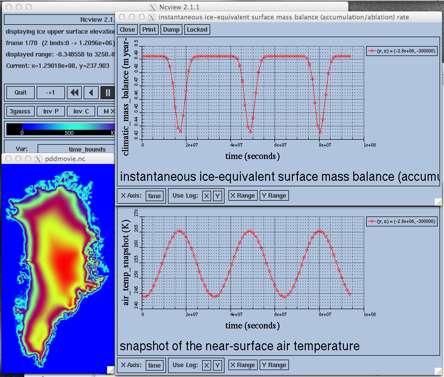
Fig. 45 Time series of the surface mass balance rate and near-surface air temperature.
We can also test the surface temperature forcing code with the following command.
pism -i g20km_10ka.nc -bootstrap \
     -surface simple \
     -atmosphere searise_greenland,delta_T \
     -atmosphere_delta_T_file pism_dT.nc \
     -spatial_times 100 -ys -125e3 -ye 0 \
     -spatial_vars ice_surface_temp \
     -spatial_file dT_movie.nc \
     -stress_balance.model none \
     -energy.model none \
     -age.enabled no \
     -geometry.update.enabled no
The output dT_movie.nc and pism_dT.nc were used to create
Fig. 46.
This figure shows the GRIP temperature offsets and the time-series of the temperature at the ice surface at a point in southern Greenland (bottom graph), confirming that the temperature offsets are used correctly.
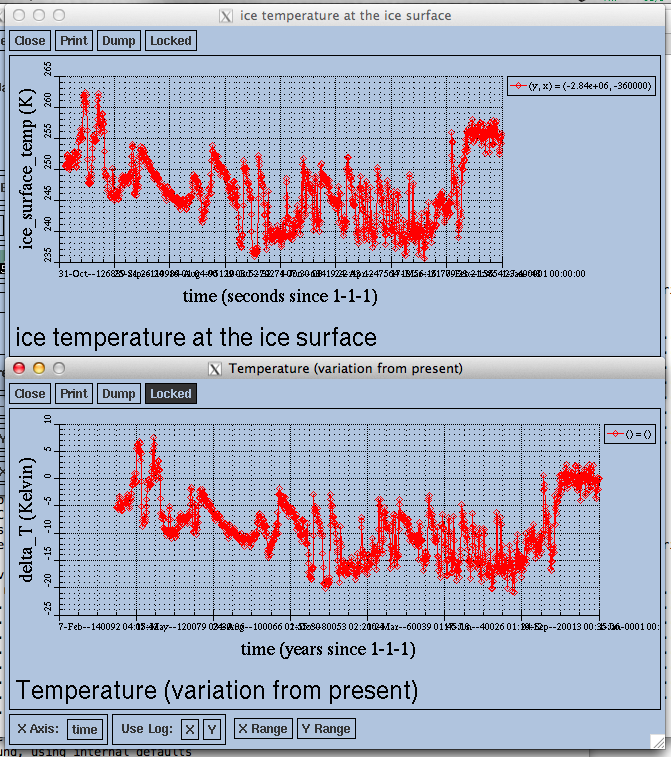
Fig. 46 Time series of the surface temperature compared to GRIP temperature offsets
| Previous | Up | Next |