Watching the first run

As soon as the run starts it creates time-dependent NetCDF files ts_g20km_10ka.nc and ex_g20km_10ka.nc. The latter file, which has spatially-dependent fields at each time, is created after the first 100 model years, a few wall clock seconds in this case. The command -extra_file ex_g20km_10ka.nc -extra_times -10000:100:0 adds a spatially-dependent “frame” at model times -9900, -9800, …, 0.

To look at the spatial-fields output graphically, do:

ncview ex_g20km_10ka.nc

We see that ex_g20km_10ka.nc contains growing “movies” of the fields chosen by the -extra_vars option. A frame of the ice thickness field thk is shown in Fig. 2 (left).

The time-series file ts_g20km_10ka.nc is also growing. It contains spatially-averaged “scalar” diagnostics like the total ice volume or the ice-sheet-wide maximum velocity (variable ice_volume_glacierized and max_hor_vel, respectively). It can be viewed by running

ncview ts_g20km_10ka.nc

The growing time series for ice_volume_glacierized is shown in Fig. 2 (right). Recall that our intention was to generate a minimal model of the Greenland ice sheet in approximate steady-state with a steady (constant-in-time) climate. The measurable steadiness of the ice_volume_glacierized time series is a possible standard for steady state (see [12], for exampe).

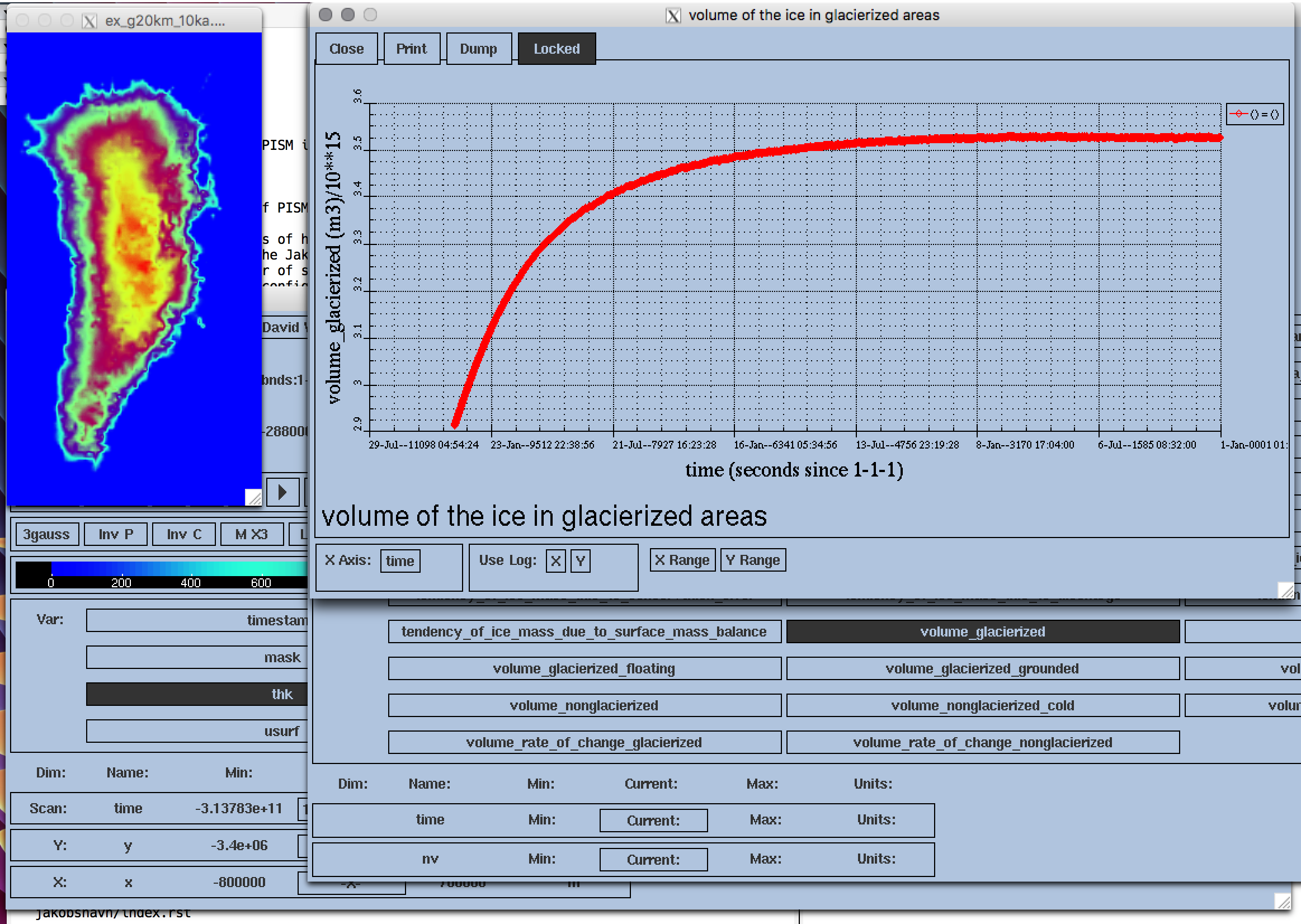
Fig. 2 Two views produced by ncview during a PISM model run.

Left

thk, the ice sheet thickness, a space-dependent field, from file ex_g20km_10ka.nc.

Right

ice_volume_glacierized, the total ice sheet volume time-series, from file ts_g20km_10ka.nc.

At the end of the run the output file g20km_10ka.nc is generated. Fig. 3 shows some fields from this file. In the next subsections we consider their “quality” as model results. To see a report on computational performance, we do:

ncdump -h g20km_10ka.nc | grep history

which prints

:history = "user@machine 2017-10-04 19:16:08 AKDT: PISM done.  Performance stats: 0.1784 wall clock hours, 0.7136 proc.-hours, 14005.0054 model years per proc.-hour.\n",

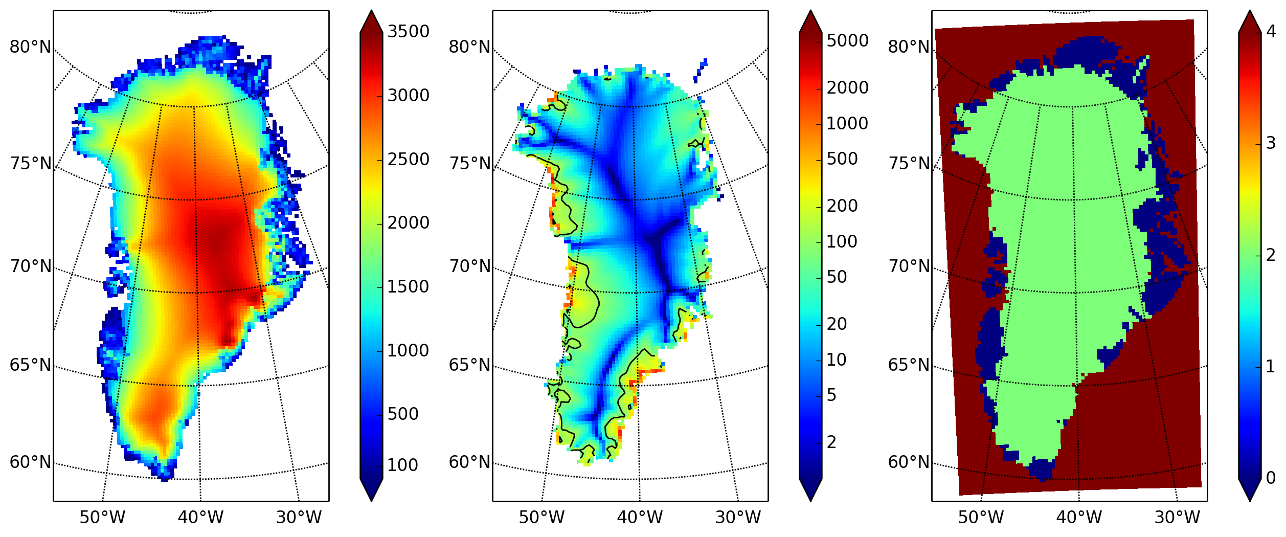
Fig. 3 Fields from output file g20km_10ka.nc.

Left

usurf, the ice sheet surface elevation in meters.

Middle

velsurf_mag, the surface speed in meters/year, including the 100 m/year contour (solid black).

Right

mask, with 0 = ice-free land, 2 = grounded ice, 4 = ice-free ocean.

---

Previous

Up

Next