Third run: higher resolution

Now we change one key parameter, the grid resolution. Model results differ even when the only change is the resolution. Using higher resolution “picks up” more detail in the bed elevation and climate data.

If you can let it run overnight, do

PARAM_PPQ=0.5 ./spinup.sh 4 const 10000 10 hybrid g10km_10ka_hy.nc &> out.g10km_10ka_hy &

This run might take 4 to 6 hours. However, supposing you have a larger parallel computer, you can change “mpiexec -n 4” to “mpiexec -n N” where N is a substantially larger number, up to 100 or so with an expectation of reasonable scaling on this grid [10], [11].

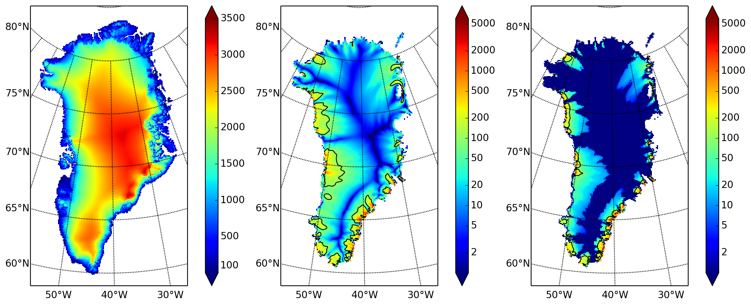
Fig. 6 Fields from output file g10km_10ka_hy.nc.

Compare to Fig. 4, which only differs by resolution.

Left

usurf in meters.

Middle

velsurf_mag in m/year.

Right

velbase_mag in m/year.

Some fields from the result g10km_10ka_hy.nc are shown in Fig. 6. Fig. 5 also compares observed velocity to the model results from 20 km and 10 km grids. As a different comparison, Fig. 7 shows ice volume time series ice_volume_glacierized for 20 km and 10 km runs done here. We see that this result depends on resolution, in particular because higher resolution grids allow the model to better resolve the flux through topographically-controlled outlet glaciers (compare [28]). However, because the total ice sheet volume is a highly-averaged quantity, the ice_volume_glacierized difference from 20 km and 10 km resolution runs is only about one part in 60 (about 1.5%) at the final time. By contrast, as is seen in the near-margin ice in various locations shown in Fig. 5, the ice velocity at a particular location may change by 100% when the resolution changes from 20 km to 10 km.

Roughly speaking, the reader should only consider trusting model results which are demonstrated to be robust across a range of model parameters, and, in particular, which are shown to be relatively-stable among relatively-high resolution results for a particular case. Using a supercomputer is justified merely to confirm that lower-resolution runs were already “getting” a given feature or result.

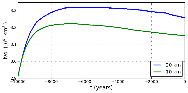
Fig. 7 Time series of modeled ice sheet volume ice_volume_glacierized on 20km and 10km grids. The present-day ice sheet has volume about \(2.9\times 10^6\,\text{km}^3\) [6], the initial value seen in both runs.

---

Previous

Up

Next